Data Science by Nicolas Pedraza

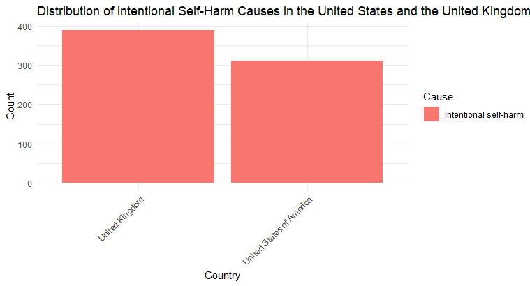
  Final Project Advanced Statistics and Analytics  Nicolas Pedraza LIS4273: Advanced Statistics and Analytics  Professor: Alon Friedman  Topic : Self-Harm and Substance Abuse Deaths Worldwide  Introduction Upon reviewing various databases I discovered this dataset on self-harm and substance abuse caught my attention due to the absence of recent statistics on the matter . Using the statistical tools learned in this course, I plan to uncover a series of questions I have about the numbers behind this dataset.  The objective is to analyze intentional self-harm and psychoactive substance use-related deaths.  The dataset, obtained from the World Health Organization Mortality Database, includes 48,631 observations and 8 variables, information on deaths categorized by Year, Cause, Age Range, ISO Code, Sex, Deaths, Age/Sex, and Country.  Hypotheses  1. Overall Trends:  There is a significant difference in self-harm deaths in the United State...

 a.  # Install and load necessary packages install.packages("ggplot2") library(ggplot2) # Create a data frame with the provided data data <- data.frame(   Month = rep(month.abb, each = 2),   Year = rep(c(2012, 2013), times = 12),   Value = c(31.9, 39.4, 27, 36.2, 31.3, 40.5, 31, 44.6, 39.4, 46.8, 40.7, 44.7,             42.3, 52.2, 49.5, 54, 45, 48.8, 50, 55.8, 50.9, 58.7, 58.5, 63.4) ) # Convert Month and Year to a date format data$Date <- as.Date(paste(data$Year, data$Month, "1", sep = "-")) # Create a time series plot ggplot(data, aes(x = Date, y = Value, group = Year, color = as.factor(Year))) +   geom_line() +   geom_point() +   labs(title = "Student Credit Card Charges Over Time",        x = "Date",        y = "Charges") +   theme_minimal() b.  # Fit an Exponential Smoothing Model fit <- ets(data$Value) # Print the statistical outcome summary(fit) c. Tim...

 10.1:  # Load the ISwR package if not already installed if (!require(ISwR)) {   install.packages("ISwR")   library(ISwR) } # Load the "ashina" data data(ashina) # Create a subject factor variable ashina$subject <- factor(1:16) # Attach the "ashina" dataset attach(ashina) # Create data frames for active and placebo treatments act <- data.frame(vas = vas.active, subject, treat = 1, period = grp) plac <- data.frame(vas = vas.plac, subject, treat = 0, period = grp) # Set up the additive model additive_model <- aov(vas ~ subject + treat + period, data = rbind(act, plac)) # Perform t-tests for treatment comparison t_test_treat <- t.test(vas.active, vas.plac, alternative = "two.sided") # View the ANOVA results summary(additive_model) # Print the t-test results print(t_test_treat) The additive model (additive_model) allows you to examine the effect of the subject, treatment, and period on the response variable (vas.active). It provides es...